Learning by interacting with our environment is omnipresent in human life. Most of the time we don't have a teacher to tell us exactly to what do in each situation. Instead, we are learning by doing and observing the outcomes of our actions. Reinforcement Learning is learning which actions to take in a given situation to maximize a reward we get from doing so. The agent must explore which actions yield the most reward by trying them out. A learner's action do not only affect the current reward but also the next state and thus all following rewards.
Reinforcement learning consists of the central two parts of exploration of actions on the one hand and exploitation of rewards on the other. Supervised learning on the other hand, the most common form of machine learning nowadays, consists of learning from a given dataset of labeled samples. To give a correct prediction in an interactive problem, the model must be given a representative and correct sample of all situations which might occur over all time steps into the future. It is most often infeasible to achieve this through pure supervised learning.
Components of Reinforcement Learning
- A policy defines which action should be taken by the agent in a given state. A policy can be deterministic (same output everytime) or stochastic (output is sampled from a probability distribution)
- At each time step, the agent receives a one-dimensional numerical reward. Maximizing the total reward an agent gains is the main target of reinforcement learning. It is the primary way of changing the policy.
- A value function predicts the total long-term reward one can expect to gain, starting from a given state.
Finite Markov Decision Processes
Markov decision processes define a framework for sequential decision-making which is used for reinforcement learning. In each state an action can be taken will yield a reward and lead to a new state which will then indirectly influence possible future rewards.
The agent is the learner and decision maker and interacts with the environment, which consists of everything outside the agent. The agent keeps selecting actions and the environment keeps responding with a new state and a reward.
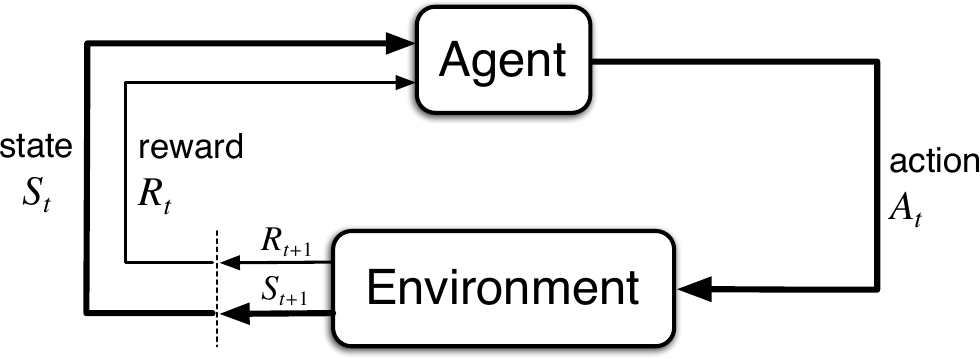 (Figure 3.1 from [1])
At each time step \(t = 0, 1, 2, ...\) the agent receives a state \(S_t \in \mathcal{S}\), selects an action \(A_t \in \mathcal{A}(s)\) and receives a numerical reward \(R_{t+1} \in \mathcal{R} \subset \mathbb{R}\)
In a finite MDP, the sets \(\mathcal{S}\), \(\mathcal{A}\), and \(\mathcal{R}\) all have a finite number of elements.
The dynamics of the MDP is the probability of ending up in a new state \(s'\) and receiving a reward \(r\) given a state \(s\) and action \(a\):
\(p(s', r | s, a) \doteq Pr\{S_t = s', R_t = r | S_{t-1}=s, A_{t-1}=a\}\)
In applications where one can define a final time step, each such subsequence of time steps is called an episode. Each episode ends in a so-called terminal state, after which a reset of the environment leads to a new start state.
The return is the discounted sum of rewards over time:
\(G_t \doteq R_{t+1} + \gamma R_{t+2} + \gamma^2 R_{t+3} + ... = \sum_{k=0}^{T} \gamma^k R_{t+k+1}\)
where \(\gamma\) with \(0 \leq \gamma \leq 1\) is the discount rate, describing the fact that immediate rewards are considered more valuable than those further in the future. Here \(T\) describe the final time step. For unepisodic cases, it would be replaced with \(\infty\). The general goal is to find the actions which result in the highest return.
Policies and Value Functions
A policy \(\pi(a|s)\) is the probability of selecting an action \(A_t = a\) if \(S_t = s\). It can be set as a rule set an agent follows.
The state-value function \(v_\pi(s)\) of a state \(s\) for a policy \(\pi\) is the expected return when starting in \(s\) and following \(\pi\) thereafter.
\(v_\pi(s) \doteq \mathbb{E}_\pi\left[G_t | S_t = s\right] = \mathbb{E}_\pi\left[\sum_{k=0}^\infty\gamma^k R_{t+k+1}| S_t = s\right]\) for all \(s \in \mathcal{S}\).
The action-value function \(q_\pi(s, a)\) is the expected return starting from state \(s\), taking action \(a\) and thereafter following the policy \(\pi\):
\(q_\pi(s, a) \doteq \mathbb{E}_\pi\left[G_t | S_t = s, A_t = a\right] = \mathbb{E}_\pi\left[\sum_{k=0}^{\infty}{\gamma^k R_{t+k+1}}|S_t=s, A_t=a\right]\)
Conclusion
There are various methods which try to improve an approximation to the value function or the action-value function to then decide which are the optimal actions to take. Other approaches directly learn an approximation of the policy. These topics will be covered in more detail in the future. This concludes the first part of my Introduction to Reinforcement Learning.
References
[1] R. S. Sutton and A. G. Barto. Reinforcement learning: An introduction. MIT Press, 2018
Comments