Introduction
The availability of compact and informative representations of sensor data is essential for robotics control and artificial intelligence (AI). In the past, these representations were created manually, but now Deep Learning provides a framework for learning them from data. This is especially important for robotics because the high-dimensional data from multiple sensors can be transformed into a much lower-dimensional state that contains only essential information for a particular task. Reinforcement learning algorithms use these low-dimensional states to learn controllers and take actions that maximize rewards.
However, finding and defining interesting states for control tasks often requires a considerable amount of manual engineering. Thus, the goal is to learn these features with as little supervision as possible. State representation learning (SRL) is a type of feature learning that focuses on transforming observations into states, which can then be used for efficient policy learning. SRL is often framed in a control setup that favors small dimensions for the state space, ideally with a semantic meaning that correlates with some physical feature. For example, a state might consist of the coordinates and the speed in each dimension of an object.
Learning in this context should be performed without explicit supervision, and the SRL literature may make use of knowledge about the physics of the world, interactions, and rewards whenever possible, serving as semi-supervision or self-supervision, which aids the challenge of learning state representations without explicit supervision. Building such models can exploit a large set of objectives or constraints, possibly taking inspiration from human learning. For example, infants expect objects to follow the principles of persistence, continuity, cohesion, and appearance-based attributes such as color and texture.
SRL is a critical technique for robotics control and AI that allows for the efficient learning of low-dimensional state representations from high-dimensional sensor data. By using information about actions, their consequences in the observation space, and rewards, along with generic constraints on what a good state representation should be, SRL can automate the feature learning process with minimal supervision.
Benefits of Model-based Reinforcement Learning
Why is a model needed at all to perform reinforcement learning? There are several motivations behind creating a model during the RL process. [1]
Data Efficiency After building a model an agent can plan in this model for a desired amount of time before acting in the environment. This allows to extract as much information as possible from a minimal number of training steps. In real world environments like robotics or autonomous driving, where performing steps is expensive this can lead to a massive increase in the data and sample efficiency. Especially if failure is expensive or even dangerous, when for example harm to humans is possible, this improvement is of great benefit.
Exploration One of the fundamental challenges of RL is the question on how to balance exploration of rewarding unvisited states with the exploitation of the parts of the environment that are already known. If no model is available, then we have much more limited opportunities on how to design our exploration. The naivest approach here is \(\epsilon\)-greedy exploration [2] where at each time step we pick one random possible action with a certain probability \(\epsilon\). In model-based approaches we have wide array of options instead. We can use different exploration strategies in planning compared to real environment steps. We can explore by following our current value estimates of states or by intrinsic motivation [3] where we define a metric on what makes a state interesting to explore, for example based on our uncertainty of the state or its novelty. We can also differ in how deep or how wide we explore the state space.
Transfer Learning Learning a model of the environment enables us to transfer this model to a similar environment, where the dynamics or the reward function differ. It also allows us to transfer knowledge learned from simulated environments into real-world environment without having the cost or risks of having to learn from scratch in the real world.
Safety Particularly for real-world applications, safety is extremely critical. A robot or a self-driving vehicle might destroy itself or other objects or hurt humans if no safeguards are in place. If we have an internal model of our surroundings and can propose estimates on which outcomes have which probability we can alleviate this. This can be done in diverse ways, for example by defining a safe region or having uncertainty estimates and verifying the safety of the current policy.
Explainability With the rise of more powerful artificial intelligence, it becomes increasingly more crucial to be able to explain their internal workings and mitigate their black-box nature [4]. By learning of a model of the environment we can make it more understandable and interpretable to a human. For example, we can learn symbolic representations, interpretable transition models, or preference models. Or we can use visual explanations like attention or have textual descriptions. Alternatively, we can use as a basis of the model specific formulas restricting the model or use fuzzy controllers [5].
Definitions
We have an agent acting in an environment. At every time step \(t\) the agent collects an observation \(o_{t}\in{\mathcal{O}}\) through its sensors and takes an action \(a_{t}\in{\mathcal{A}}\) where \({\mathcal{O}}\) is the observation space and \({\mathcal{A}}\) is either a discrete or continuous action space. This leads to a state transition from the current state to the next state.
In the reinforcement learning setting, the agent receives a reward \(r_t\) defined by a reward function designed to steer the agent towards optimal behavior.
The goal of State Representation Learning (SRL) is to learn a representation \(s_t \in \mathcal{S}\) where \(\mathcal{S}\) is the representation state space. We learn a mapping \(\phi\) from the history of observations \(o_{1:t}\), actions \(a_{1:t}\) and rewards \(r_{1:t}\) until time step \(t\) to the representation:
We are interested in the case where we don't have access to the true state and thus need to rely on unsupervised or self-supervised learning. This process often involves predicting a reconstruction of the observation, denoted by \({\hat{o}}_{t}\) and analogously we can reconstruct actions with \({\hat{a}}_{t}\) and rewards with \({\hat{r}}_{t}\).
Types of Models
Forward Model A forward model predicts the next state \(s_{t+1}\) given a current state \(s_t\) and action \(a_t\). It is the most widely used model for lookahead planning. First, we encode the information from \(o_t\) to \(s_t\), followed by generating a prediction for the next state \(\hat{s}_{t+1}\). We can also put constraints on it, such as linear dynamics between \(s_t\) and \(s_{t+1}\). The forward model equation can be represented as
To learn the model, the error between the predicted state \(\hat{s}_{t+1}\) and the actual next state \(s_{t+1}\) is backpropagated through both the transition and encoding models.
Inverse Model Given a state \(s_t\) and a next state \(s_{t+1}\), (or observations \(o_t\) and \(o_{t+1}\)) the inverse model predicts which action \(a_t\) would lead to the transition. Again, we encode observations to receive the state representations, then predict the action:
This way, the state can be designed to hold enough information to retrieve the action that caused the modification.
Backward Model In a backward model, we predict which previous state \(s_{t-1}\) and previous action \(a_{t-1}\) led to a given state \(s_{t}\) (or observation \(o_{t}\))
This we way can plan in the backwards direction.
Frequently Used Approaches
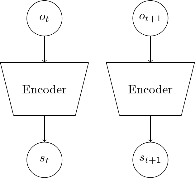
Siamese networks
Siamese networks [6] consist of multiple networks that are identical and share parameters, meaning that they have the same weights. The purpose of siamese architecture is not to categorize input data but to differentiate between inputs (for example, determining whether they belong to the same or different classes or conditions). This type of architecture is beneficial for imposing restrictions on the latent space of a neural network.
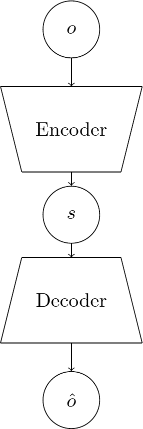
Auto-encoders (AEs)
Auto-encoders consist of an encoder which maps the input into a latent space and a decoder which maps this latent representation back into the original input space. They are frequently utilized to acquire state representations and are widely employed for reducing the dimensionality of data. In our particular situation, we denote the input as \(o_t\) the latent representation as \(s_t\) and the reconstructed output as \({\hat{o}}_{t}\) The dimension of the latent representation is determined by the dimension of the state representation we want to learn, and it can be constrained if necessary. The AE automatically learns a compact representation by minimizing the reconstruction error between input and output. The usual metric used to measure the reconstruction error is the mean squared error (MSE) between input and output, calculated pixel-wise, but other losses can also be employed.
Denoising auto-encoders
A regular AE can be thought of as learning to compress and reconstruct an observation. Depending on the size and quality of the given dataset, a regular AE might find a solution that is too simple and does not generalize well. Denoising auto-encoders [7] [8] have the same basic structure and loss function as auto-encoders. Differently, in their training process random noise is added to each observation which needs to be removed in the reconstruction. This leads to a more robust encoder and decoder.
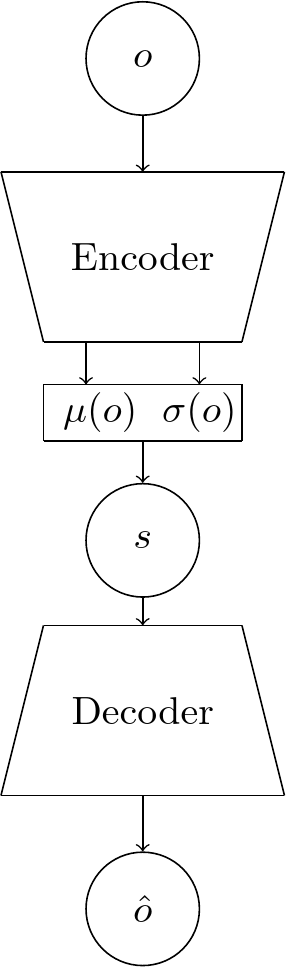
Variational auto-encoders (VAEs)
A variational auto-encoder [9] is an auto-encoder which maps the input to the parameters of a probability distribution of \(o_t\). This means we can interpret the encoder as distribution \(p_\theta(s_{t}|o_{t})\) from which the states in \(\mathcal{S}\) are sampled from, which we approximate with \(q_{{\phi}}{\big(}s_{t}{\big|}o_{t}{\big)}\), where \(\phi\) are the parameters of the encoder. Similarly, the decoder represents the distribution \(p_\theta(o_{t}|s_{t})\) and \(\theta\) are the parameters of the decoder. Usually, the latent distribution is assumed to be a multivariate Gaussian with zero-mean and diagonal covariance:
There are two parts of the loss when training a VAE. Firstly, as in the regular AE, we have a reconstruction error (usually in the form of a mean-squared error). Secondly, there is a regularization error which tries to keep the latent distribution close to the prior distribution.
Once trained, VAEs can be used generate new data, by sampling from this latent distribution of \(s_t\) and then decoding it.
This basic version of the variational auto-encoder can be extended to versions which work on sequences of inputs, see for example [10-21]. These approaches will be discussed in more detail in a future article.
Summary
This concludes a first overview over the motivation and the building blocks of model learning and state representation learning. In the next part, we will look at the core challenges, loss functions, and evaluation methods.
References
[1] T. M. Moerland, et al. Model-based Reinforcement Learning: A Survey. 2022
[2] R. S. Sutton and A. G. Barto. Reinforcement learning: An introduction. 2018
[3] N. Chentanez, A. G. Barto and S. Singh. Intrinsically Motivated Reinforcement Learning. 2004
[4] G. Vilone and L. Longo. Explainable artificial intelligence: a systematic review. arXiv preprint arXiv:2006.00093. 2020
[5] C. Glanois, et al. A Survey on Interpretable Reinforcement Learning. arXiv preprint arXiv:2112.13112. 2021
[6] S. Chopra, R. Hadsell and Y. LeCun. Learning a Similarity Metric Discriminatively, with Application to Face Verification. 2005 IEEE Computer Society Conference on Computer Vision and Pattern Recognition (CVPR'05), 1. 539-546. 2005
[7] P. Vincent, et al. Extracting and composing robust features with denoising autoencoders. Proceedings of the 25th international conference on Machine learning - ICML '08. 1096-1103. 2008
[8] P. Vincent, et al. Stacked denoising autoencoders: Learning useful representations in a deep network with a local denoising criterion. Journal of machine learning research, 11. 2010
[9] D. P. Kingma and M. Welling. Auto-Encoding Variational Bayes. arXiv preprint arXiv:1312.6114. 2013
[10] M. Watter, et al. Embed to Control: A Locally Linear Latent Dynamics Model for Control from Raw Images. arXiv: Learning. 2015
[11] J. Bayer and C. Osendorfer. Learning Stochastic Recurrent Networks. ArXiv. 2014
[12] R. G. Krishnan, U. Shalit and D. Sontag. Deep kalman filters. arXiv preprint arXiv:1511.05121. 2015
[13] J. Chung, et al. A recurrent latent variable model for sequential data. Advances in neural information processing systems, 28. 2015
[14] M. Fraccaro, et al. Sequential neural models with stochastic layers. Advances in neural information processing systems, 29. 2016
[15] R. Krishnan, U. Shalit and D. Sontag. Structured Inference Networks for Nonlinear State Space Models. Proceedings of the AAAI Conference on Artificial Intelligence, 31. 2017
[16] M. Fraccaro, et al. A Disentangled Recognition and Nonlinear Dynamics Model for Unsupervised Learning. Advances in neural information processing systems, 30. 3601-3610. 2017
[17] M. Karl, et al. Deep Variational Bayes Filters: Unsupervised Learning of State Space Models from Raw Data. arXiv preprint arXiv:1605.06432. 2017
[18] A. Goyal, et al. Z-Forcing: Training Stochastic Recurrent Networks. ArXiv. 2017
[19] W. Hsu, Y. Zhang and J. R. Glass. Unsupervised Learning of Disentangled and Interpretable Representations from Sequential Data. 2017
[20] Y. Li and S. Mandt. Disentangled Sequential Autoencoder. 2018
[21] S. Leglaive, et al. A Recurrent Variational Autoencoder for Speech Enhancement. ICASSP 2020 - 2020 IEEE International Conference on Acoustics, Speech and Signal Processing (ICASSP). 371-375. 2020
Comments