Variational Autoencoders for State Space Models

Introduction

In the last article we have introduced state space models and how to extend the concept of the variational auto-encoder to them and how to train them. We will now look at several examples of VAEs for SSMs in more detail.

Deep Kalman Filter

The Deep Kalman Filter [1] is based on the same graphical model as the Kalman Filter described above. But instead, neural networks are used to encode the information into a latent space and decode it back into the original dimension.

ssm_example

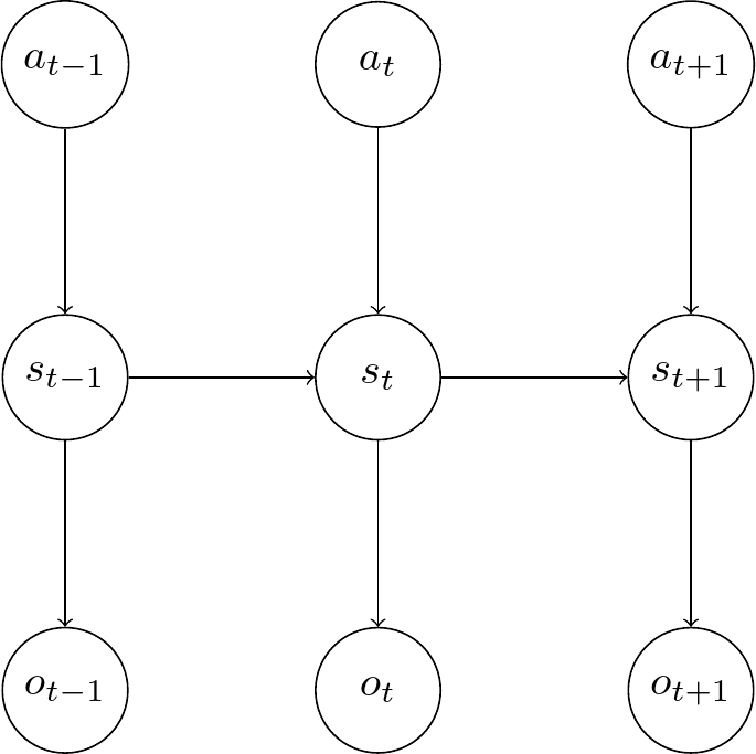
According to the rules of d-separation we can observe that the $s_{t-1}$ node separates all observations $o_{<t}$, actions $a_{<t}$ from $s_t$. Or more formally, $s_t \perp o_i|s_{t-1}$ and $s_t \perp a_i|s_{t-1}$ for $i < t$ such that the posterior distribution simplifies to

$$p_{\theta}\left(\mathbf{s}_{1:T}\mid\mathbf{o}_{1:T},\mathbf{a}_{1:T}\right)=\prod_{t=1}^{T}p_{\theta}\left(\mathbf{s}_{t} \mid \mathbf{s}_{t-1},\mathbf{o}_{t:T},\mathbf{a}_{t:T}\right)$$

Similarly, we can deduce the following simplifications:

$$p_\theta\left({\bf o}_{t}\vert{\bf o}_{1:t-1},{\bf s}_{1: t},{\bf a}_{1: t}\right)=p_\theta\left({\bf o}_{t}\vert{\bf s}_{t}\right)$$

$$p_\theta\left(\mathbf{s}_{t}|\mathbf{o}_{1:t-1},\mathbf{s}_{1:t-1},\mathbf{a}_{1:t}\right)=p_\theta \left(\mathbf{s}_{t}|\mathbf{s}_{t-1},\mathbf{a}_{t}\right)$$

Therefore, the VLB becomes

$$\mathcal{L}(\theta,\phi;{\bf o}_{1:T},{\bf a}_{1:T}) = \sum_{t=1}^{T}{\mathbb{E}_{q_{\phi}({\bf s}_{1:T}|{\bf o}_{1:T},{\bf a}_{1:T})}\big[\log p_\theta({\bf o}_{t}\vert{\bf s}_{t})\big]} -$$

$$- \sum_{t=1}^{T}{\mathbb{E}_{q_{\phi}({\bf s}_{1:T}|{\bf o}_{1:T},{\bf a}_{1:T})}\big[D_{\mathrm{KL}}\big( q_\phi(\mathbf{s}_{t}|\mathbf{s}_{t-1},\mathbf{o}_{t:T},\mathbf{a}_{t:T})\parallel\ p_{\theta}(\mathbf{s}_{t}|\mathbf{s}_{t-1},\mathbf{a}_{t})\big)\big]}$$

Krishnan et al. [1] proposed four different neural network models which represent approximations to different probability distributions: - A neural network for the current state, observation, and action $q_\phi({\bf s}_t|{\bf o}_{t},{\bf a}_{t})$ - A neural network for the recent past and future $q_\phi({\bf s}_t|{\bf o}_{t-1:t+1}, {\bf a}_{t-1:t+1})$ - An RNN modelling the complete past $q_\phi({\bf s}_t|{\bf o}_{1:t},{\bf a}_{1:t})$ - An RNN modelling the whole sequence $q_\phi({\bf s}_t|{\bf o}_{1:T},{\bf a}_{1:T})$

Deep Variational Bayes Filter

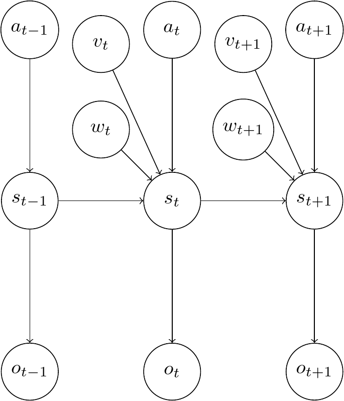
The Deep Variational Bayes Filter [2] modifies the graphical model to include stochastic parameters $\beta_t$, which consists of two added terms $v_t$ and $w_t$. The former is a noise parameter independent of the input, the latter is noise depending on the input. It is a regularizing prior on the

The transition model is assumed to depend on these parameters and factorize in the following way, where $s_t$ only depends on the previous state $s_{t-1}$ and no other states as well:

$$p({\bf s}_{1:T}\mid\beta_{1:T},{\bf a}_{1:T})=\prod_{t=1}^{T}p({\bf s}_{t}\mid{\bf s}_{t-1},{\bf a}_{t},\beta_{t})$$

For the observation model the assumption is made that the current state $s_t$ contains all necessary information about the current observation $o_t$:

$$p({\bf o}_{1:T}\mid{\bf s}_{1:T},{\bf a}_{1:T})=\prod_{t=1}^{T}p({\bf o}_{t}\mid{\bf s}_{t})$$

The approximate recognition model is designed as:

$$q_{\phi}({\bf{\beta}}_{1:T}\mid{\bf o}_{1:T})=q_{\phi}({\bf w}_{1:T}\mid{\bf o}_{1:T})\,q_{\phi}({\bf v}_{1:T})$$

dvbf-graphical-model

The VLB of a DVBF is derived as

${\mathcal{L}}_{\mathrm{DVBF}}(\mathbf{o}_{1:T},\theta,\phi\mid\mathbf{a}_{1:T}) = \mathbb{E}_{q_{\phi}}[\log p_{\theta}(\mathbf{o}_{1:T}\mid\mathbf{s}_{1:T})]-D_{\mathrm{KL}}(q_{\phi}(\beta_{1:T}\mid\mathbf{o}_{1:T},\mathbf{a}_{1:T})\mid p(\beta_{1:T}))$

Where again, the first term is a reconstruction error, and the second term is a regularization term to keep the approximate distribution close to the prior of $\beta_{1:T}$.

How the transitions themselves and the parameters $w_t$ look like, can be chosen according to the application. For example, one approach is to model a locally linear transition model, where the filter learns a number of transition matrices similar to a Kalman filter and weighing parameters $\alpha_i$ to arrive at the final matrices as a linear combination of these matrices. But nonlinear-transitions can be implemented as well.

An example implementation of a DVBF with locally linear transitions can be found here: https://github.com/gregorsemmler/pytorch-dvbf

Variational Recurrent Neural Networks

In Variational Recurrent Neural Networks [3] we have internal determinstic states $h_t$, denoted by a diamond shape in the graphical model, and implemented with an RNN.

vrnn-graphical-model-v2-fixed

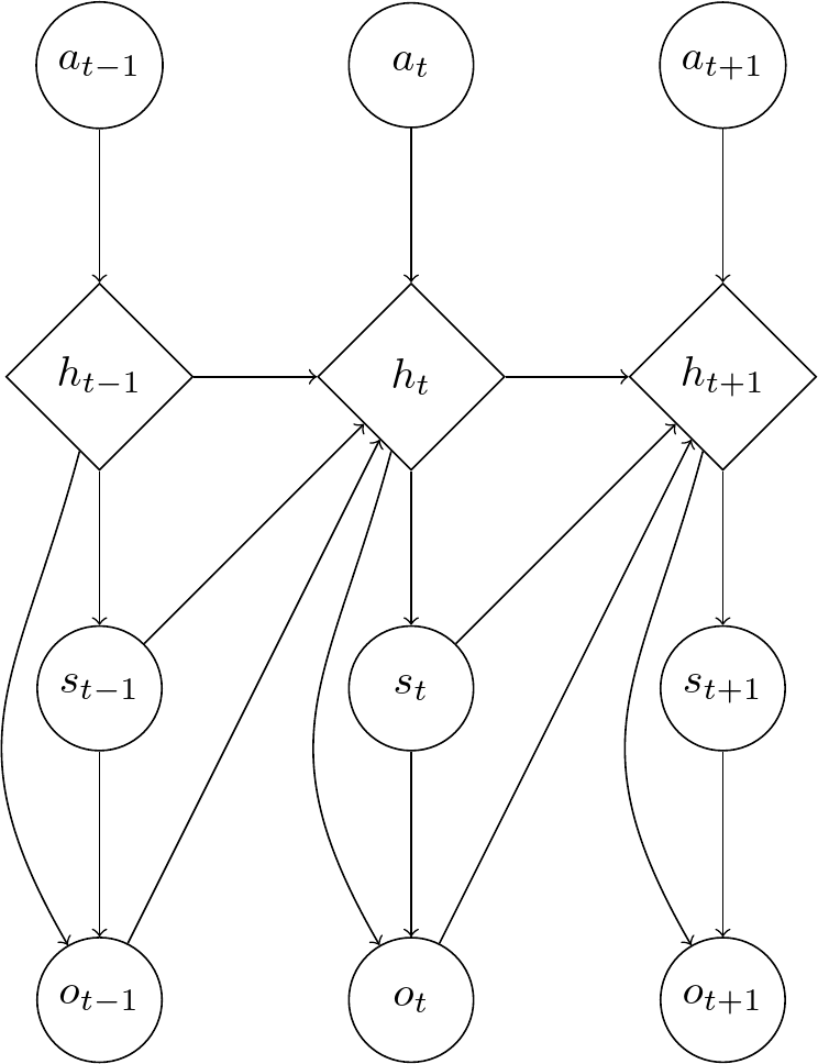
We start with an initial internal state $h_1$ and action $a_1$ from which the first state $s_1$ is generated, after which $o_1$ is induced from the previous two. Then we get $h_2$ from $a_2$, $h_1$, and $s_1$ and the second state $s_2$ from $s_1$ and the process continues in that manner.

The $h_i$ values can be defined as a deterministic function $f$ of the other random variables. We can write

$${\bf h}_t = f\big({\bf o}_{t-1}, {\bf s}_{t-1}, {\bf a}_t, {\bf h}_{t-1}\big)$$

If we unroll this recursively, we get the function $g$

$${\bf h}_t = f\big({\bf o}_{t-1}, {\bf s}_{t-1}, {\bf a}_t, f\big({\bf o}_{t-2}, {\bf s}_{t-2}, {\bf a}_{t-1}, \ldots f\big({\bf o}_0, {\bf s}_0, {\bf a}_1, {\bf h}_0\big)\big)\big) \triangleq g\big({\bf o}_{1:t-1}, {\bf s}_{1:t-1}, {\bf a}_{1:t}\big)$$

Where $o_0, s_0, h_0$ are treated as special initialization values and not part of the actual graphical model.

The joint distribution can be represented as

$$p_\theta\big({\bf o}_{1:T}, {\bf s}_{1:T}, {\bf a}_{1:T}, {\bf h}_{1:T}\big) = \prod_{t=1}^T p_\theta\big({\bf o}_t \mid {\bf s}_t, {\bf h}_t\big) p_\theta\big({\bf s}_t \mid {\bf h}_{t}\big) p_\theta\big({\bf h}_t \mid {\bf o}_{t-1}, {\bf s}_{t-1}, {\bf a}_{t}, {\bf h}_{t-1} \big) p_\theta\big({\bf a}_t\big)$$

With

$$p_\theta\big({\bf h}_t \mid {\bf o}_{t-1}, {\bf s}_{t-1}, {\bf a}_{t}, {\bf h}_{t-1} \big) = \delta \big({\bf h}_t; f\big({\bf o}_{t-1}, {\bf s}_{t-1}, {\bf a}_t, {\bf h}_{t-1}\big) \big)$$

where $\delta \big(h_t; x \big)$ is the dirac delta which is $1$ at position $x$, otherwise $0$.

To retrieve the joint distribution without the deterministic nodes, we can marginalize them out

$$p_\theta\big({\bf o}_{1:T}, {\bf s}_{1:T}, {\bf a}_{1:T}\big) = \int_{-\infty}^{\infty}\ldots\int_{-\infty}^{\infty}p_\theta\big({\bf o}_{1:T}, {\bf s}_{1:T}, {\bf a}_{1:T}, {\bf h}_{1:T}\big) d{\bf h}_1\ldots d{\bf h}_T =$$

$$= \int \ldots\int \prod_{t=1}^T p_\theta\big({\bf o}_t \mid {\bf s}_t, {\bf h}_t\big) p_\theta\big({\bf s}_t \mid {\bf h}_{t}\big) \delta \big({\bf h}_t; f\big({\bf o}_{t-1}, {\bf s}_{t-1}, {\bf a}_t, {\bf h}_{t-1}\big) \big) p_\theta\big({\bf a}_t\big) d{\bf h}_1\ldots d{\bf h}_T$$

$$= \prod_{t=1}^T p_\theta\big({\bf o}_t \mid {\bf s}_t, g\big({\bf o}_{1:t-1}, {\bf s}_{1:t-1}, {\bf a}_{1:t}\big)\big) p_\theta\big({\bf s}_t \mid g\big({\bf o}_{1:t-1}, {\bf s}_{1:t-1}, {\bf a}_{1:t}\big)\big) p_\theta\big({\bf a}_t\big) =$$

As $g$ is deterministic, this is equivalent to

$$= \prod_{t=1}^T p_\theta\big({\bf o}_t \mid {\bf o}_{1:t-1}, {\bf s}_{1:t-1}, {\bf a}_{1:t}\big) p_\theta\big({\bf s}_t \mid {\bf s}_{1:t-1}, {\bf o}_{1:t-1}, {\bf a}_{1:t}\big) p_\theta\big({\bf a}_t\big)$$

This means we can draw an equivalent graphical model without the deterministic nodes $h_t$

vrnn-graphical-model-v2-no-h

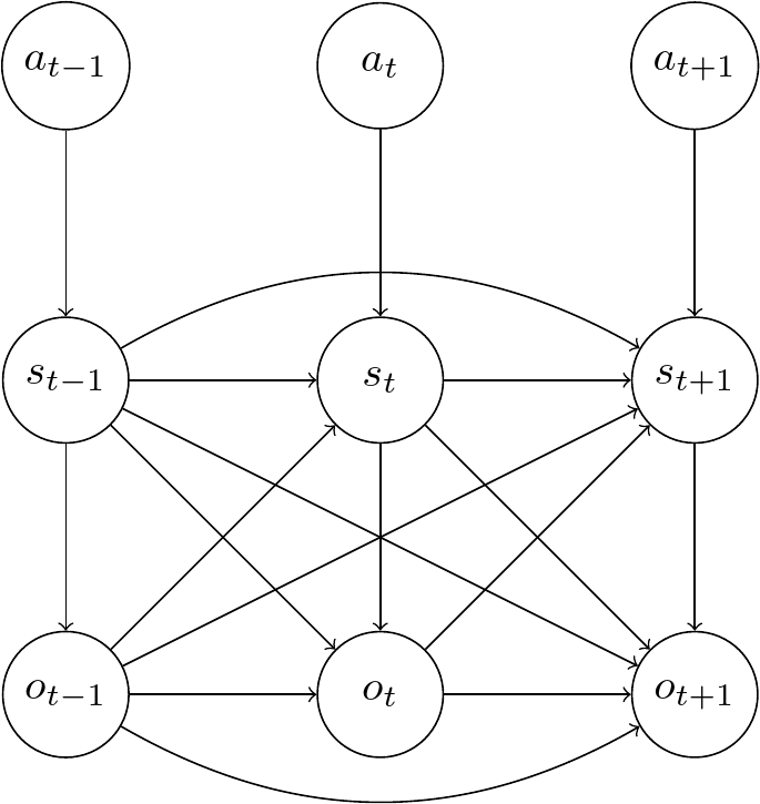
Based on this simplified graph, we can retrieve the inference model

$$p_{\theta}\left({\bf s}_{1:T}\mid\mathbf{o}_{1:T},\mathbf{a}_{1:T}\right) = \prod_{t=1}^T p_\theta\big({\bf s}_t \mid {\bf s}_{1:t-1}, {\bf o}_{1:T}, {\bf a}_{1:t}\big) $$

No further simplifications can be made according to d-separation.

This can be approximated with

$$q_{\phi}({\bf s}_{1:T}|{\bf o}_{1:T})=\prod_{t=1}^{T}q_{\phi}\bigl({\bf s}_{t}|{\bf o}_{t},{\bf h}_{t}\bigr) = \prod_{t=1}^{T}q_{\phi}\bigl({\bf s}_{t}|{\bf o}_{t},g\big({\bf o}_{1:t-1}, {\bf s}_{1:t-1}, {\bf a}_{1:t}\big)\bigr) =$$

$$= \prod_{t=1}^{T}q_{\phi}\bigl({\bf s}_{t}|{\bf s}_{1:t-1}, {\bf o}_{1:t}, {\bf a}_{1:t}\bigr)$$

For the training, we can initially observe in the graphical model(s) that there are no conditional independence assumptions made. So we would use the general VLB for VAEs for sequences as defined in a preceding section:

$$\mathcal{L}(\theta,\phi;{\bf o}_{1:T},{\bf a}_{1:T})= \sum_{t=1}^{T}{\mathbb{E}_{q_{\phi}({\bf s}_{1:T}|{\bf o}_{1:T},{\bf a}_{1:T})}\big[\log p_\theta({\bf o}_{t}\vert{\bf o}_{1:t-1},{\bf s}_{1:t},{\bf a}_{1:t})\big]} -$$

$$ - \sum_{t=1}^{T}{\mathbb{E}_{q_{\phi}({\bf s}_{1:T}|{\bf o}_{1:T},{\bf a}_{1:T})}\big[D_{\mathrm{KL}}\big( q_\phi({\bf s}_t|{\bf s}_{1:t-1}, {\bf o}_{1:T},{\bf a}_{1:T})\parallel\ p_{\theta}({\bf s}_t|{\bf o}_{1:t-1},{\bf s}_{1:t-1},{\bf a}_{1:t})\big)\big]}$$

Using the previous approximation for $q_{\phi}({\bf s}_{1:T}|{\bf o}_{1:T})$ this becomes

$$ - \sum_{t=1}^{T}{\mathbb{E}_{q_{\phi}({\bf s}_{1:T}|{\bf o}_{1:T},{\bf a}_{1:T})}\big[D_{\mathrm{KL}}\big( q_\phi({\bf s}_t|{\bf s}_{1:t-1}, {\bf o}_{1:t},{\bf a}_{1:t})\parallel\ p_{\theta}({\bf s}_t|{\bf o}_{1:t-1},{\bf s}_{1:t-1},{\bf a}_{1:t})\big)\big]}$$

Summary

In this article, we have looked at several variational auto-encoders for state space models in detail. All of them try to learn internal state representations of observations from an environment. This concludes this first series on model learning and state representation learning for model-based reinforcement learning.

References

[1] R. G. Krishnan, U. Shalit and D. Sontag. Deep kalman filters. arXiv preprint arXiv:1511.05121. 2015

[2] M. Karl, et al. Deep Variational Bayes Filters: Unsupervised Learning of State Space Models from Raw Data. arXiv preprint arXiv:1605.06432. 2017

[3] J. Chung, et al. A recurrent latent variable model for sequential data. Advances in neural information processing systems, 28. 2015

Comments