Although reinforcement learning1 has achievement remarkable, superhuman results in various applications like AlphaGo these applications have always been in simulated environments where one training run can be done and restarted quickly, and safely. In fact, these training runs can also be massively parallelized depending on the available computing resources. However, it is generally more difficult to make an approach work in a real-world application.
In those cases there are two main approaches:
- Simulate the environment as closely as possible, solve the problem in the simulation, then apply this solution to the real situation.
- Try to solve the problem in the real world application itself, as efficiently as possible based on the actually gathered data.
Firstly, in a particular application there might not be the time or the resources to make an accurate simulation of the real situation. Secondly, there is often a gap between simulation and reality where even the smallest deviation in the simulation can lead to significantly different outcomes.
For sample-efficient approaches, we will therefore consider the second solution, in particular using model-based reinforcement learning such that, in this case, a robot can learn on its own to drive in just a few trials.
Model-Based Reinforcement Learning
Model-based methods primarily use a model to plan, while model-free methods use learning. A model of the environment is everything the agent can use to predict how the environment will respond to its actions. Given a state and action, the model predicts the next state (and optionally) the next reward. The model can be used to simulate interactions and produce simulated experience. Planning here describes any approach which takes a model as input and produces, or improves a policy for the actual interaction with the environment.
Here, states are defined as \(s \in \mathbb{R}^{d_s}\) and the actions as \(a \in \mathbb{R}^{d_a}\). The dynamics function \(f_\theta : \mathbb{R}^{d_s + d_a} \mapsto \mathbb{R}^{d_s}\) of the environment maps the current state \(s_t\) and the action \(a_t\) to a new state \(s_{t+1}\) such that \(s_{t+1} = f\left(s_t,a_t\right)\). Assuming probabilistic dynamics, \(s_{t+1}\) will be given by the conditional distribution \(\mathrm{Pr}(s_{t+1}|s_t, a_t; \theta)\).
The dynamics are learned by finding an approximation \(\tilde{f}\) of the true transition function \(f\), given the dataset \(\mathbb{D} = \left\{(s_n, a_n), s_{n+1}\right\}_{n=1}^N\).
In general, this model can then be used to predict how the environment will change over the following time steps und use this to optimize over which actions to take to achieve the highest return. With a probabilistic dynamics model \(\tilde{f}\) we get a distribution over the possible future state trajectories \(s_{t:t+T}\).
Probabilistic Neural Network Ensembles
An ensemble consists of a set of multiple machine learning models. A probabilistic neural network is a network that parameterizes a probability distribution, which allows sampling from. On the other hand, a deterministic neural network gives a point prediction, so every input will always result in the same output.
The loss function used here is the negative log likelihood
\(\mathrm{loss}_P(\theta) = - \sum_{n=1}^{N} \mathrm{log}\:\tilde{f}_\theta(s_{n+1}|s_n, a_n)\).
In this case, we will have the neural networks parameterize a multivariate Gaussian distribution with diagonal covariances, so \(\mathrm{Pr}(s_{t+1}|s_t, a_t; \theta) = \mathcal{N}\left(\mu_\theta(s_t, a_t), \Sigma_\theta(s_t, a_t)\right)\) meaning the loss is the Gaussian negative log likelihood:
\(\mathrm{loss}_\mathrm{Gauss}(\theta) = \sum_{n=1}^N \left[\mu_\theta(s_n, a_n) - s_{n+1}\right]^\mathsf{T}\Sigma^{-1}_\theta(s_n, a_n)\left[\mu_\theta(s_n, a_n) - s_{n+1}\right] + \mathrm{log}\:\mathrm{det}\:\Sigma_\theta(s_n, a_n)\) ([2])
In the following example we can see a sine curve (blue) being approximated by a probabilistic neural network ensemble with 5 members trained with this loss.
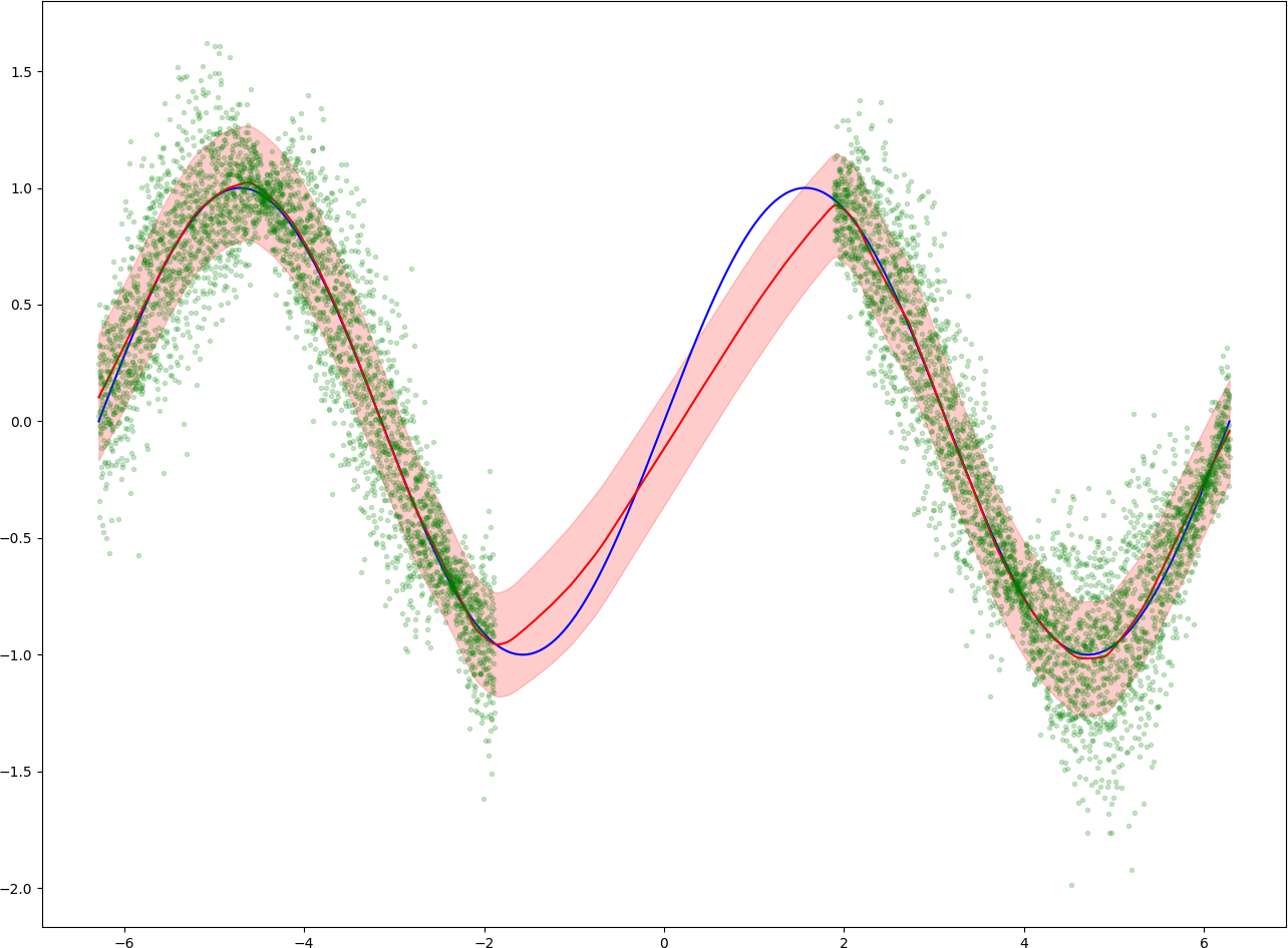
The green dots represent the training data, parts of the original data with added random gaussian noise. The red line represents the mean of the ensemble prediction, while the shaded red area represent one standard deviation around the prediction. One can see that the mean of the prediction is fairly accurate for the areas where lots of training data is available, while deviating further in the middle of the plot where it isn't.
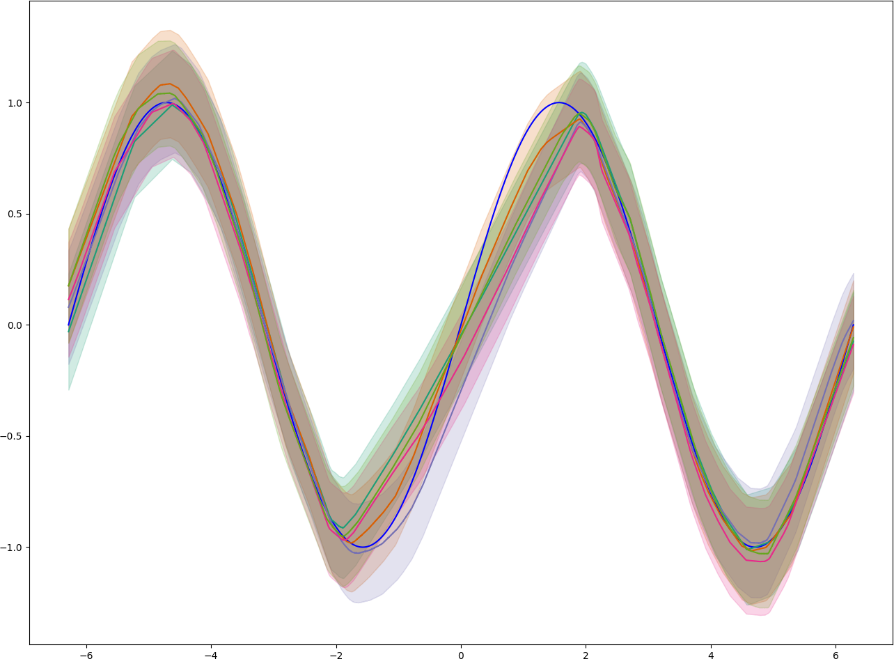
In the second plot, we can see the predictions from each member of the ensemble. Every ensemble member was trained on a subset of the training data which results in differing predictions.
Trajectory Sampling
The classic approach from dynamic programming to update a model of the environment is to perform sweeps over the state or state-action space, updating each once per sweep. On tasks with a large state-space this would take an unfeasible long time. Complete sweeps spend equal time on all parts of the state space, instead of putting more focus on important states.
The second approach is to sample from the state or state-action space from some probability distribution. An intuitive solution is to sample from the one which is observed from the current policy. Which means starting from the start state we interact with the model and keep simulating until an end state is reached. The transitions are given by the model and actions are given by the current policy. This way of generating updates is called trajectory sampling.
In this context, one can create multiple particles from a state, and keep simulating until a terminal state is reached. If trajectory sampling is performed on an ensemble, for each ensemble member multiple particles can be propagated and then the final results are amalgamated. This is the basic idea behind probabilistic ensemble trajectory sampling (PETS), one method we will be examining in more detail here. The central optimization within this algorithm is the Cross-Entropy Method (CEM).
Cross-Entropy Method (CEM) Optimizer
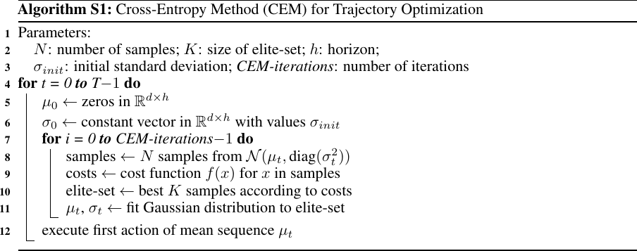 (image from [3])
The Cross-Entropy Method (CEM) is a stochastic and derivative-free optimization method, meaning it can solve problems without needing backpropagation. The CEM optimizer takes initial parameters \(\mu_0, \sigma_0\) for a normal distribution. In each iteration, multiple samples are taken from the current distribution \(\mathcal{N}(\mu_t, \mathrm{diag}(\sigma_t^2))\) which are inputs to a cost function. An elite set of the best performing samples are then used to update the current solution.
Probabilistic Ensemble Trajectory Sampling
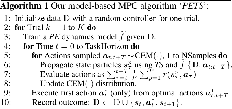 (image from [2])
In simple terms, the PETS algorithm follows the following steps: At the beginning of each trial, train a probabilistic ensemble dynamics model \(\tilde{f}\) given the currently available dataset. Then, repeat for each step in the trial:
- Sample actions \(a_{t:t+T}\) from the current CEM distribution.
- Propagate the states particles \(s_\tau^p\) through the ensemble given the actions using trajectory sampling.
- Get the average rewards over the particles and time steps: \(\sum_{\tau=t}^{t+T} \frac{1}{P} \sum_{p=1}^P r(s_\tau^p, a_\tau)\)
- Update the CEM distribution according to the best performing actions.
- Perform the first action \(a_t^*\) from the CEM solution which we consider the optimal action.
- Add the state, action, next state, (and optionally reward) to the dataset.
This is repeated until the desired return is achieved or a set number of trials is done.
Practical Experiment
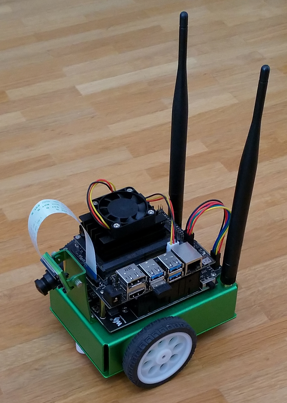
To evaluate the approach, I am trying to get a robot to drive on its own. For this I am using a JetBot. It is based on the Nvidia Jetson Nano Developer Kit.
The most important technical features are:
| Feature | Description |
|---|---|
| GPU | 128-core Maxwell |
| CPU | Quad-core ARM A57 @ 1.43 GHz |
| Memory | 4 GB 64-bit LPDDR4 25.6 GB/s |
| Video Encode | 4K @ 30, 4x 1080p @ 30, 9x 720p @ 30 (H.264/H.265) |
The robot has two wheels controlled by two independent motors, a mounted camera and two wireless antennas. The operating system is Ubuntu 18.04.
The task for the robot is to learn to drive on a mat without driving off. The traction of the wheels on the floor turned out to be too low by comparison.
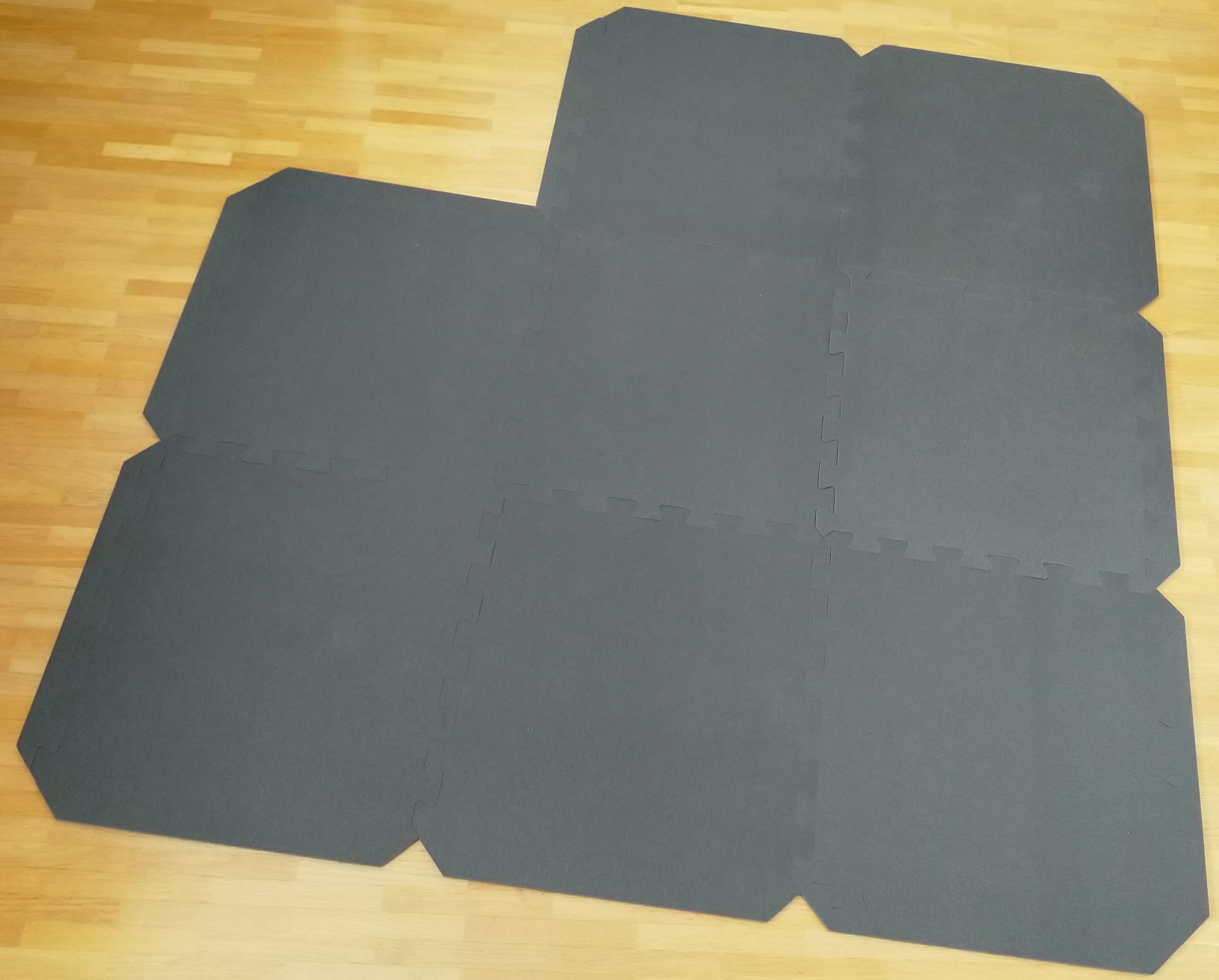
A separate classification model was trained to detect if the robot is driving off the mat, which is used to determine whether one episode is over.
The reward is calculated as the amount of forward motor activation minus a threshold times a constant factor. The maximum speed is capped at \(a_{max} = 0.15\) to avoid the robot from being damaged. This means the main task the robot gets is to drive forward (without leaving the mat).
\(r(s, a) = (a_l + a_r - 2 * a_{thresh}) * val_{mul}\)
Where \(a = (a_l, a_r)\) and \(a_l\), \(a_r\) are the speed values for the left and the right motor and the \(a_{thresh}\) is a threshold which the motor speed needs to have at minimum. The robot doesn't move forward if the speed is too low, the robot might learn to just stand still in that case. The values were \(a_{thresh} = 0.1\) and \(val_{mul} = 10\).
The only sensor input of the robot are raw camera input images with a width and height of 224 and 3 channels. For this reason, an Autoencoder was trained on a dataset of about 60,000 frames. The encoder then encodes the input down to a dimension of 512, which is used as the input to the PETS algorithm. The robot was also limited to forward movements, as there is no camera in the back.
The ensemble was made out of 5 neural networks, each consisting of two fully-connected layers with 512 members and the ELU activation function.
The Adam optimizer with a learning rate of 1e-3 was used to train the ensemble for 5 epochs before each trial. In total, 10 trials were performed.
For the CEM Optimizer, 500 samples were taken from the ensemble with 20 particles each, which were propagated 30 time steps into the future. The optimization was done for 5 iterations at each time step to get the final action to be taken.
As only a few trials were performed, the replay buffer of size 25000 was never full, so all previous samples were used in each training run.
Results
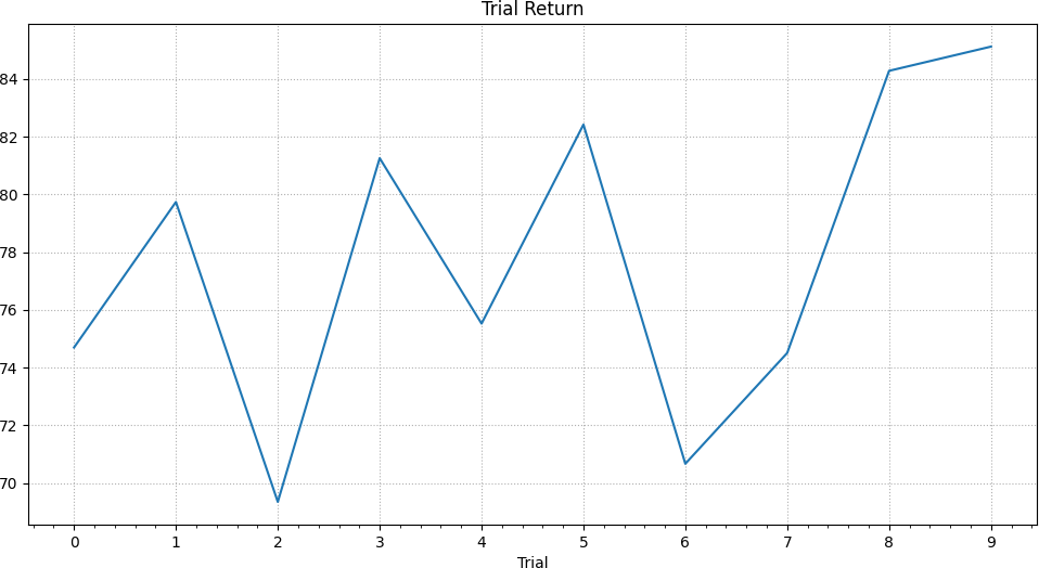
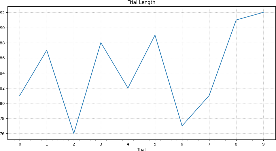
After 10 trials, the robot has successfully learned to drive forward based on the given inputs and reaches its highest return reward of 85.12 in the final trial. This is orders of magnitudes faster than classic methods which can easily take hundreds or thousands of episodes.
At this point, the robot has only learned to drive forward as the reward function gives the highest reward for doing so, while a penalty is given if a motor is moving too slow. For this reason, taking a turn is also penalized, and as there is no penalty for ending the trial it has learned to rather drive to the end of the mat than to change course. A differently designed reward function would offset this behavior, for example by not penalizing slow motor activation.
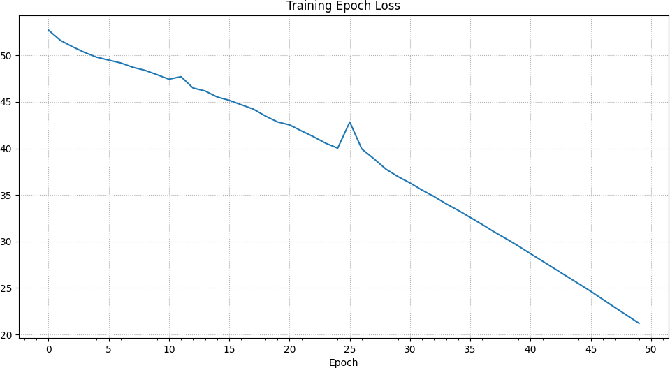
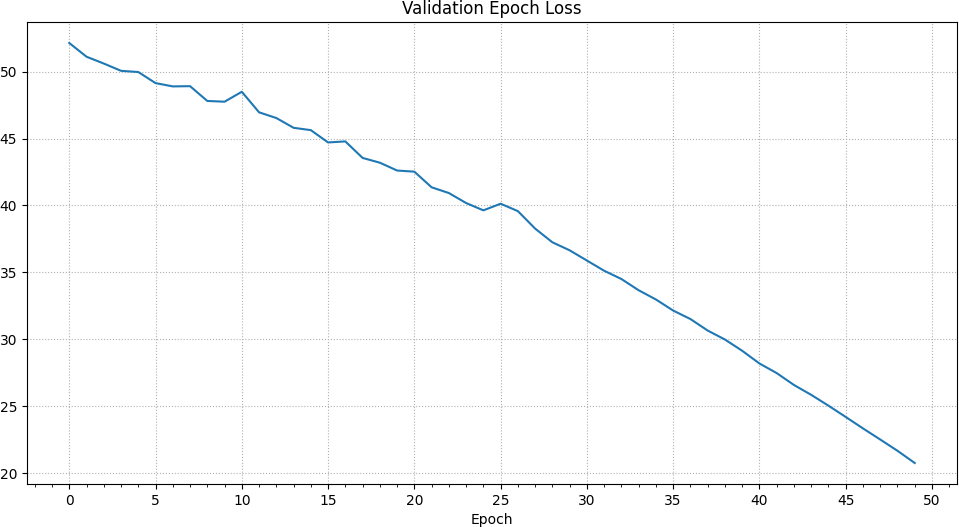
The loss is steadily reduced over all epochs with a slight spike at the 25th epoch.
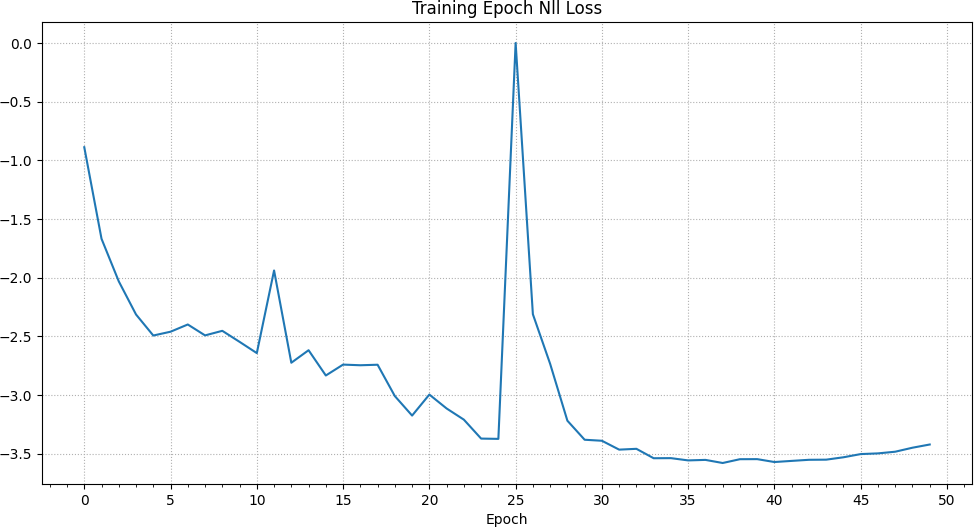
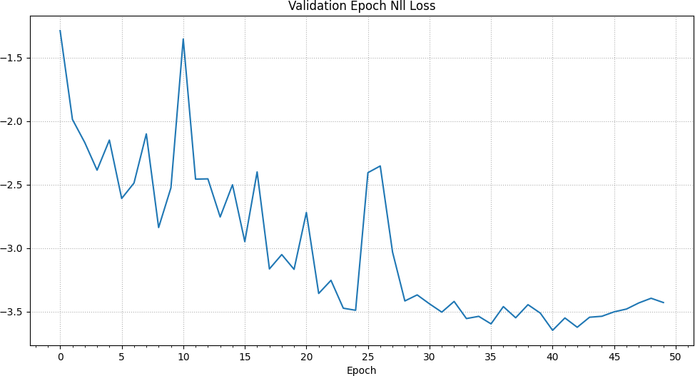
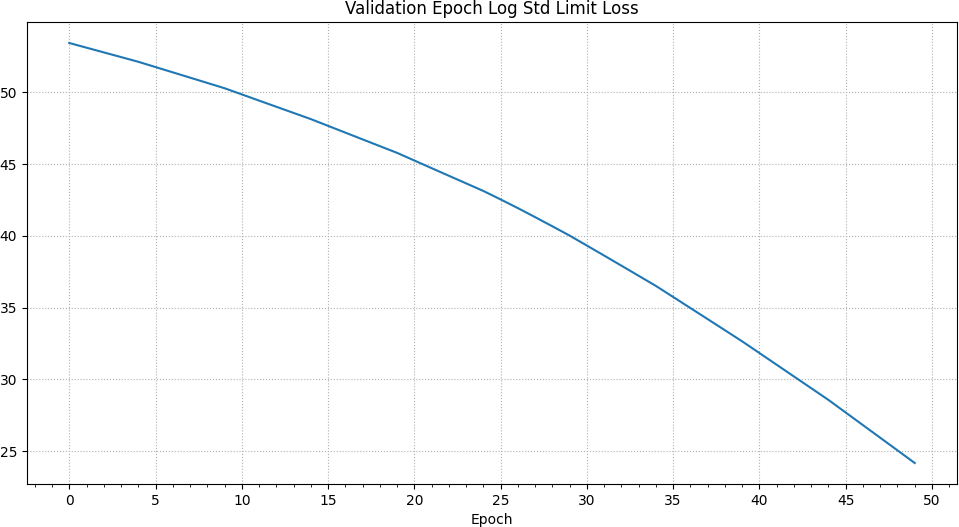
In addition to the previously described negative log likelihood loss, there is an additional loss which allows the ensemble to learn limits to its output standard deviation / variance.2 This method was also described by the authors of the original PETS paper. It is also worthy of note that the nll loss can reach negative values. Once again, we can see a spike in the training nll loss at the 25th epoch up to a value close to 0 and otherwise a continuing decrease.
Videos
Initially the robot drives randomly over the mat:

In less than ten trials it has learned to drive forward on the mat:

We can conclude that the robot has learned to drive forward to maximize rewards. However, it has not yet learned to drive through a curve. One reason for this is, that the reward function is maximized by driving forward, while a curve is punished, as one of the wheels is not driving forward. No reward is lost by driving to the edge ending the trial. Instead, the penalty for driving curves could be removed and a negative reward for the end of the trial added. This would encourage more of a circular motion, while staying on the mat. Alternatives to the CEM optimizer can also be considered for improved results.
Summary
This concludes my first introduction into sample efficient model-based reinforcement learning by presenting how the PETS algorithm can be used to help a robot to learn to drive by itself in less than 10 trials, based only on raw input images and a reward function in each state. On my GitHub profile I have provided my implementation of the algorithm.
References
[1] R. S. Sutton and A. G. Barto. Reinforcement learning: An introduction. MIT Press, 2018.
[2] K. Chua, et al. Deep reinforcement learning in a handful of trials using probabilistic dynamics models. Advances in neural information processing systems, 2018
[3] C. Pinneri, et al. Sample-efficient cross-entropy method for real-time planning. arXiv preprint arXiv:2008.06389, 2020.
Footnotes
- See also my introduction to reinforcement learning ↩
- See here for how the standard deviation is limited in my implementation. ↩
Comments