For visual tasks, humans and animals alike put more focus on certain parts of an observed scene. For example, when given the task to detect whether a given image of an animal displays or a dog or cat, one might focus at the nose, eyes or ears. Convolutional neural networks have achieved remarkable results in various applications in recent years. However, for a human observer it is mostly incomprehensible how the neural network has come to its conclusion, therefore not allowing deeper analysis of both correct and incorrect outputs. If we could teach a machine learning model to learn to pay attention to specific parts of an input image it would allow us to interpret which parts are deemed most important, leading to a more interpretable and explainable process.
Attention
For this, we can use scalar matrices which show the relative importance of specific parts of the image for the given task, so-called attention maps. For image classification, for example, the attention can determine the location of the object of interest. There are different ways to implement attention, either as a trainable mechanism or as an analysis after the fact.
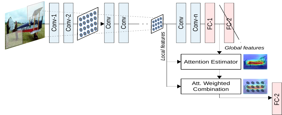
In this case we will look at a method by Jetley et al. [1] which includes attention estimators integrated into different points of the CNN architecture.
 (Image from [1])
The local features refer to the outputs from a convolutional layer within the network, while the global features refer to the outputs of the last layer before the final classification layer. The local features therefore have a receptive field for some local part of the image while the global features have the complete image has a receptive field. Each attention estimator has as input both local and global features.
 (Image from [1])
In a CNN the convolutional layers closer to the input will learn to extract abstract features like edges while later layers will capture increasingly complicated shapes. By positioning attention maps at different points in the network structure we can capture the spatial location of important parts of the image at different levels of abstraction.
The idea is to find relevant areas in the image and increasing their importance while decreasing the influence of insignificant ones. Through the restriction of the attention modules the network has to learn a compatibility between the local feature vectors from the middle parts of the network and the global feature vector. It has to use a combination of the local and global features based on learned compatibility scores.
Here we will use a compatibility score function \(\mathcal{C}\)
\(c_i^s = \left\langle u, l_i^s + g \right\rangle,\: i \in \{1, ..., n \}\)
where \(\langle\cdot\rangle\) is the dot product between the two vectors. Instead of concatenating the \(l_i^s\) and \(g\), addition is used, to simplify the process [1].
In a usual CNN the global image descriptor \(g\) is derived from the input image and passed through a final fully connected layer (used for classification for example). The network must learn to map the input into a higher dimensional space (via the CNN) layers, before then getting back to the final output. In this method, the layers are encouraged to learn similar mappings between the local descriptors \(l_i\) and the global descriptor \(g\) at multiple stages in the CNN pipeline. A local descriptor is only able to contribute to the final step in proportion to the compatibility with the global descriptor \(g\). This means that only parts of the image important for the global task should result in a high compatibility score.
SqueezeNet
In a previous article I have discussed how a robot can learn to drive in less than ten trials. There are different neural networks used in this application.
The first one is a classification network which detects whether the robot is on the mat and thus if the episode is over. Because we want to save resources on our JetBot we want to consider small and efficient models.
One famous mobile model is SqueezeNet [2], a model which manages to reach the accuracy of AlexNet [3] on the ImageNet image dataset with a size of only about 0.5 MiB.
 (image from [2])
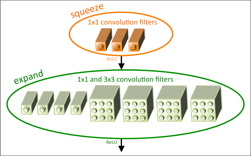
The central part of the model architecture is the fire module which consists of a squeeze and an expand step. The squeeze convolution layer only has 1x1 filters after which the ReLU activation is used and the values are expanded back with 1x1 and 3x3 convolutional filters, followed by a final ReLU activation. The usage of this module helps keep the model size down while keeping high performance.
Augmenting the model architecture

Similar to the VGG example above, we can extend the SqueezeNet architecture (left) by adding multiple attention modules to it (right).
The architecture consists of one initial and one final convolutional layer, intermediate max pool operations and otherwise of fire modules which allow to capture increasingly more complex shapes while keeping the model size down. We add the attention modules after the first convolutional layer, and the second and fourth fire module, before the following max pool layers. The global output (out of the adaptive average pool layer a_avg_pool) and the outputs of the attention modules are concatenated together and are input into the final linear layer.
Visualization
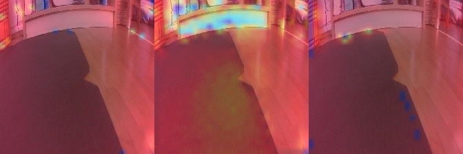
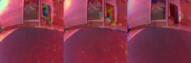
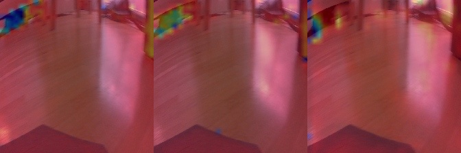
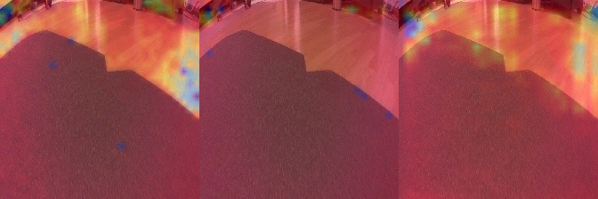
We can visualize the three attention maps (left to right corresponding to the first, second and last) produced for an image via a heatmap. Blue colors indicate less attention and red colors more. The compatibility scores sum up to 1 over all pixels.
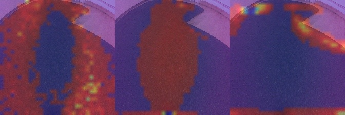
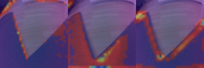
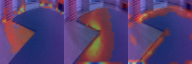
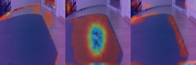
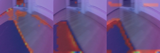
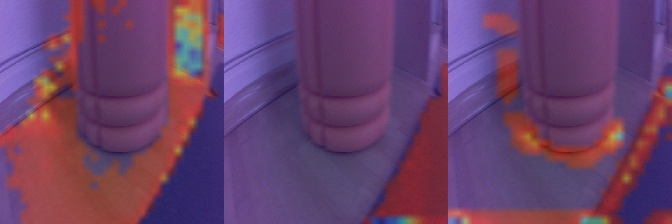
For the classification network which detects whether the robot is on the mat, we can see that the middle and especially the right attention module put more emphasis attention to the edges of the mat and try to find other edges in the case where the mat is not visible. For the attention map closest to the input on the left we can see that broader areas on the ground receive the most attention.
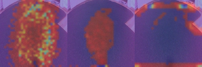
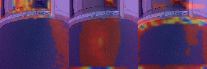
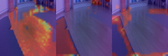
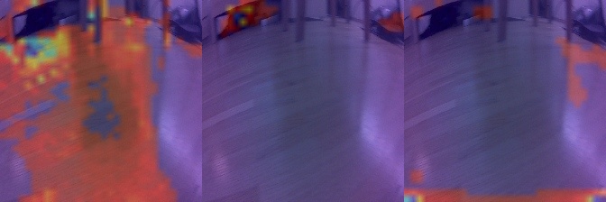
The next network to be considered is the encoder part of the autoencoder used to compress the input images down to the latent dimension. Again, we can use the attention squeezenet network.
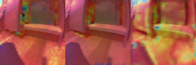
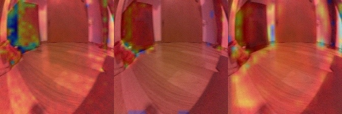
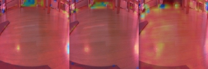
Interestingly we can see that in general, for all attention maps, the network gives about the same amount of attention to all areas of the input image. Intuitively, we can say that the autoencoder needs to do that to be able to reconstruct the original image as well as possible via the decoder.
Conclusion
In this article we examined a way to visualize what a convolutional neural network pays attention to enable a more explainable approach for a human and less of a black box model. This allows examining what a model uses in both correct and incorrect predictions. We can also determine that for different tasks, the model learns to pay attention to different parts of the image. For classification, the model pays attention to the edges of the mat, because that is most important to detect if the robot is driving off the mat. For the encoding model, all parts of the image are paid attention to equally, as they need to be reconstructed as accurately as possible by the decoder. If further constraints are put into the encoding process, we can expect the attention to reflect that, accordingly.
References
[1] S. Jetley, et al. Learn to pay attention. arXiv preprint arXiv:1804.02391, 2018.
[2] F. N. Iandola, et. al. SqueezeNet: AlexNet-level accuracy with 50x fewer parameters and \(<\)0.5MB model size. arXiv preprint arXiv:1602.07360, 2016.
[3] A. Krizhevsky, I. Sutskever, and G. E. Hinton. Imagenet classification with deep convolutional neural networks. Communications of the ACM, 2017, 60.6, 84-90.
Comments