State Space Models and Variational Inference

Introduction

In the last article we have looked at VAEs, how to train them and the concept of directed graphical models to represent relationships between random variables. Now we will look at state space models, an application of directed graphical models to portray sequences of random variables and how to extend the principles of VAEs to them.

State Space Models

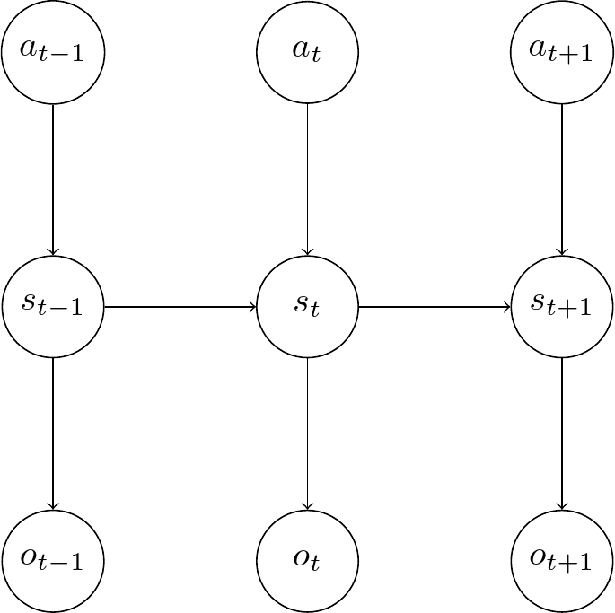
State space models (SSM) consists of several types of real-valued random variables. Here, we denote the hidden real-valued variables as $s_t$, the input variables (action) as $a_t$, and the output variables $o_t$ (which are the reconstructed observations) for each discrete-valued time step $t$. They can be represented as directed graphical models, where each node represents a random variable, and an edge represents a conditional dependency [1].

Kalman Filter

A special case are linear-gaussian SSMs [1], also known as linear dynamical systems. In this case, the transition and observation models are linear, with added Gaussian noise. In particular, the transition model has the form

$$\mathbf{s}_{t}=\mathbf{A}_{t}\mathbf{s}_{t-1}+\mathbf{B}_{t}\mathbf{a}_{t}+ {\mathcal{N}}(\mathbf{0},\mathbf{Q}_{t})$$

And the observation model has the form

$$\mathbf{o}_{t}=\mathbf{C}_{t}\mathbf{s}_{t}+\mathbf{D}_{t}\mathbf{a}_{t}+ {\mathcal{N}}(\mathbf{0},\mathbf{R}_{t})$$

Where $\mathbf{A_t, B_t, C_t, D_t, Q_t, R_t}$ are matrices of appropriate size. If they are independent of the time, the model is called stationary and we can drop the time index $t$. Often, we model the observations to only be dependent on the latent variables, so in this case the second equation simplifies to

$$\mathbf{o}_{t}=\mathbf{C}_{t}\mathbf{s}_{t} + {\mathcal{N}}(\mathbf{0},\mathbf{R}_{t})$$

Combined with a stationary model we get the transition model

$$\mathbf{s}_t =\mathbf{A} \mathbf{s}_{t-1}+\mathbf{B}\mathbf{a}_{t}+ {\mathcal{N}}(\mathbf{0},\mathbf{Q})$$

and observation model

$$\mathbf{o}_{t}=\mathbf{C} \mathbf{s}_{t} + {\mathcal{N}}(\mathbf{0},\mathbf{R})$$

We can represent this as a graphical model:

ssm_example

The kalman filter allows to solve this exactly. We can predict the hidden state $s_t$ based on the history of the previous observations $\mathbf{o_{1:t-1}}$ and actions $\mathbf{a_{1:t}}$ [1].

$$p(\mathbf{s}_{t}|\mathbf{o_{1:t-1}},\mathbf{a_{1:t}}) = {\mathcal{N}}(s_{t}|\mu_{t},\Sigma_{t}) = \int_{-\infty}^{\infty} \mathcal{N}(\mathbf{s}_{t}|\mathbf{A}_{t}\mathbf{s}_{t-1}+\mathbf{B}_{t}\mathbf{a}_{t},\mathbf{Q}_{t})\mathcal{N}(\mathbf{s}_{t-1}|\mu_{t-1},\mathbf{\Sigma}_{t-1})d\mathbf{s}_{t-1}$$

Variational Autoencoders for State Space Models

The original VAE does not contain temporal information, so the encoder learns a latent representation where each data point is independent of its time index $t$, so no transition information is contained. Several works have tried to extend the unsupervised representation learning to correlated temporal sequences in the years after [2-12]. These approaches all vary in how they define the dependencies between the observed and latent variables and their generative and inference models. Recurrent neural networks are also used as part of the generative and inference models. But all models use the basic VAE approach of an inference model and the maximization of a variational lower bound. They all also use continuous latent random variables and use discrete time steps of observed and latent random vectors.

Learning

We now consider models which handle the case where we have a sequence of observations $o_{1:T}$, of latent variables (or states) $s_{1:T}$, and (optionally) of actions $a_{1:T}$. In general, we assume that the variables within those sequences are correlated with each other. The structure of the dependencies of the variables is usually written as a product of conditional distributions using the chain rule. Here, the different orderings can be chosen which allows for different sampling processes and implementations. Often it is assumed that the distribution of a variable at time $t$ only depends on other variables of time $t$ or earlier.

We usually assume that the actions are deterministic, so we are interested only interested in the distributions over the observations and latent variables. So, we can model the joint distribution of observations and latent variables, conditioned on the actions according to the chain rule, following the time steps $t$, as [13]

$$p({\bf o}_{1:T},{\bf s}_{1:T}\vert{\bf a}_{1:T})=\prod_{t=1}^{T}p({\bf o}_{t},{\bf s}_{t}\vert{\bf o}_{1:t-1},{\bf s}_{1:t-1},{\bf a}_{1:t}) =$$

$$= \prod_{t=1}^{T}p({\bf o}_{t}\vert{\bf o}_{1:t-1},{\bf s}_{1:t},{\bf a}_{1:t})p({\bf s}_{t}\vert{\bf o}_{1:t-1},{\bf s}_{1:t-1},{\bf a}_{1:t})$$

The implementation is done with a combination of feedforward neural networks and recurrent neural networks (RNNs). The latter are used to capture the aggregated previous data (for example the past states). How this works is that an internal state variable $h_t$ of the RNN is computed at each time step $t$. We can denote such implementations by including deterministic nodes in our graphical model for these state variables.

According to the chain rule, the posterior distribution of the hidden states can be written as

$$p_{\theta}(\mathbf{s}_{1:T} | \mathbf{o}_{1:T},\mathbf{a}_{1:T})=\prod_{t=1}^{T}p_{\theta}(\mathbf{s}_{t}|\mathbf{s}_{1:t-1},\mathbf{o}_{1:T},\mathbf{a}_{1:T})$$

Depending on the conditional dependencies of the model, this can be simplified.

The VLB in this case can be derived analogously to the standard VAE case above. Combined with the above factorization, we arrive at

$$\mathcal{L}(\theta,\phi;{\bf o}_{1:T},{\bf a}_{1:T})=\mathbb{E}_{q_{\phi}({\bf s}_{1:T}|{\bf o}_{1:T},{\bf a}_{1:T})}\big[\log p_{\theta}({\bf o}_{1:T},{\bf s}_{1:T}|{\bf a}_{1:T}) - \log q_{\phi}({\bf s}_{1:T}|{\bf o}_{1:T},{\bf a}_{1:T})\big] = $$

$$= \sum_{t=1}^{T}{\mathbb{E}_{q_{\phi}({\bf s}_{1:T}|{\bf o}_{1:T},{\bf a}_{1:T})}\big[\log p_\theta({\bf o}_{t}\vert{\bf o}_{1:t-1},{\bf s}_{1:t},{\bf a}_{1:t})\big]} -$$

$$ - \sum_{t=1}^{T}{\mathbb{E}_{q_{\phi}({\bf s}_{1:T}|{\bf o}_{1:T},{\bf a}_{1:T})}\big[D_{\mathrm{KL}}\big( q_\phi({\bf s}_t|{\bf s}_{1:t-1}, {\bf o}_{1:T},{\bf a}_{1:T})\parallel\ p_{\theta}({\bf s}_t|{\bf o}_{1:t-1},{\bf s}_{1:t-1},{\bf a}_{1:t})\big)\big]}$$

Again, the first addend can be interpreted as a construction error and the second as a regularization error. In contrast to a VAE, both terms are intractable and need to be estimated, for example with a Monte Carlo sampling approach.

Summary

We have now introduced the concept of state space models and derived the general loss function we can use for extended versions of a VAE, designed for state space models and sequences of random variables. In the next article, we will cover several examples of these in more detail.

References

[1] K. P. Murphy. Machine learning: a probabilistic perspective. 2012

[2] J. Bayer and C. Osendorfer. Learning Stochastic Recurrent Networks. ArXiv. 2014

[3] R. G. Krishnan, U. Shalit and D. Sontag. Deep kalman filters. arXiv preprint arXiv:1511.05121. 2015

[4] J. Chung, et al. A recurrent latent variable model for sequential data. Advances in neural information processing systems, 28. 2015

[5] M. Fraccaro, et al. Sequential neural models with stochastic layers. Advances in neural information processing systems, 29. 2016

[6] R. Krishnan, U. Shalit and D. Sontag. Structured Inference Networks for Nonlinear State Space Models. Proceedings of the AAAI Conference on Artificial Intelligence, 31. 2017

[7] M. Fraccaro, et al. A Disentangled Recognition and Nonlinear Dynamics Model for Unsupervised Learning. Advances in neural information processing systems, 30. 3601-3610. 2017

[8] M. Karl, et al. Deep Variational Bayes Filters: Unsupervised Learning of State Space Models from Raw Data. arXiv preprint arXiv:1605.06432. 2017

[9] A. Goyal, et al. Z-Forcing: Training Stochastic Recurrent Networks. ArXiv. 2017

[10] W. Hsu, Y. Zhang and J. R. Glass. Unsupervised Learning of Disentangled and Interpretable Representations from Sequential Data. 2017

[11] Y. Li and S. Mandt. Disentangled Sequential Autoencoder. 2018

[12] S. Leglaive, et al. A Recurrent Variational Autoencoder for Speech Enhancement. ICASSP 2020 - 2020 IEEE International Conference on Acoustics, Speech and Signal Processing (ICASSP). 371-375. 2020

[13] L. Girin, et al. Dynamical variational autoencoders: A comprehensive review. arXiv preprint arXiv:2008.12595. 2020

Comments

State Space Models and Variational Inference

Introduction