Variational Inference and Directed Graphical Models

Introduction

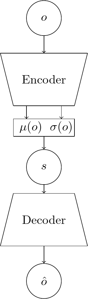
Previously, we have looked at the general idea of learning a model. One way of learning a model and state representation is through variational inference. In the context of neural networks, the variational auto-encoder [1] is the most common way of doing this. Recall that a variational auto-encoder consists of an encoder and a decoder, similar to a regular auto-encoder. In contrast though, the encoder maps to the parameters of a probability distribution, usually a multivariate normal distribution with diagonal covariance.

vae_schema

Learning for VAEs

For our unsupervised learning of the dataset, we want to approximate the true distribution of the dataset $p^*(o)$ with that of our model $p_\theta(o)$. The Kullback-Leibler (KL) divergence measures how different one probability distribution is from another. For two discrete probability distributions $p$ and $q$ of $x$ it is defined as

$$D_{\mathrm{KL}}(p\mid\mid q)=\sum_{x}p(x)\log\biggl({\frac{p(x)}{q(x)}}\biggr)$$

For two continuous distributions $p$ and $q$ of $x$ it is defined as

$$D_{\mathrm{KL}}(p\mid\mid q)=\int_{-\infty}^{\infty}p(x)\log\left(\frac{p(x)}{q(x)}\right)d x$$

We can also write

$$D_{\mathrm{KL}}(p\mid\mid q)=\mathbb{E}_{p(\mathrm{x})}\big[\log p(\mathrm{x})-\log q(\mathrm{x})\big]$$

So, we want to minimize the Kullback-Leibler (KL) divergence between these two distributions. This measurement is always greater or equal to $0$ and is $0$ if the true distributions are equal.

In our case we therefore want to minimize

$$\operatorname*{min}_{\theta}\left\{D_{\mathrm{KL}}(p^{\ast}(o)\parallel\ p_{\theta}(o))\right\}$$

which is equivalent to

$$\operatorname*{max}_{\theta}\left\{\mathbb{E}_{p^{\ast}(o)}\big[\log p_{\theta}(o)\big]\right\}$$

By doing a few restatements we get

$$\log p_{\theta}(\mathrm{o}) = \mathbb{E}_{q_\phi(s|o)}\big[\log p_{\theta}(o) \big]= \mathbb{E}_{q_\phi(s|o)}\big[ \log\left(\frac{p_{\theta}(o,s)}{p_{\theta}(s|o)}\right)\big] = $$

$$= \mathbb{E}_{q_\phi(s|o)}\big[\log q_\phi(s|o) + \log p_{\theta}(o,s) - \log p_{\theta}(s|o) - \log q_\phi(s|o) \big] = $$

$$ = \mathbb{E}_{q_\phi(s|o)}\big[\log q_\phi(s|o) - \log p_{\theta}(s|o)\big] + \mathbb{E}_{q_\phi(s|o)}\big[\log p_{\theta}(o,s) - \log q_\phi(s|o) \big] = $$

$$ = D_{\mathrm{KL}}\big( q_\phi(s|o)\parallel\ p_{\theta}(s|o)\big) + \mathcal{L}(\theta,\phi;o) $$

Where $\mathcal{L}(\theta,\phi;o)$ is the so-called evidence lower bound (ELBO) or variational lower bound (VLB) or negative variational free energy for which holds

$$\mathcal{L}(\theta,\phi;o) = \mathbb{E}_{q_\phi(s|o)}\big[\log p_{\theta}(o,s) - \log q_\phi(s|o) \big] \leq \log p_{\theta}(\mathrm{o})$$

Because, as mentioned above, for the KL divergence holds

$$D_{\mathrm{KL}}\big( q_\phi(s|o)\parallel\ p_{\theta}(s|o)\big) \geq 0$$

So, we can restate our earlier optimization problem as

$$\operatorname*{max}_{\theta}\left\{\mathcal{L}(\theta,\phi;o)\right\}$$

We can also rephrase the VLB in the form

$$\mathbb{E}_{q_\phi(s|o)}\big[\log p_{\theta}(o,s) - \log q_\phi(s|o) \big] = \mathbb{E}_{q_\phi(s|o)}\big[\log p_{\theta}(o|s) + \log p_{\theta}(s) - \log q_\phi(s|o) \big] = $$

$$= \mathbb{E}_{q_\phi(s|o)}\big[\log p_{\theta}(o|s)\big] - \mathbb{E}_{q_\phi(s|o)}\big[\log q_\phi(s|o) - \log p_{\theta}(s) \big] = $$

$$= \mathbb{E}_{q_\phi(s|o)}\big[\log p_{\theta}(o|s)\big] - D_{\mathrm{KL}}\big( q_\phi(s|o)\parallel\ p_{\theta}(s)\big) $$

Here, the first addend can be interpreted as a reconstruction error which captures the average accuracy of the whole pass through the encoder and then the decoder. The second can be seen as a regularization error that keeps the approximate distribution $q_\phi(s|o)$ close to the prior distribution over the latent variables $p_{\theta}(s)$.

For a dataset of observations $\mathrm{O}$ of size $N$ the total VLB is the sum over all the datapoints $o_n$

$$\mathcal{L}(\theta,\phi;\mathrm{O}) = \sum_{i=1}^{N} \mathbb{E}_{q_\phi(s_i|o_i)}\big[\log p_{\theta}(o_i,s_i) - \log q_\phi(s_i|o_i) \big] = $$

$$= \sum_{i=1}^{N} \mathbb{E}_{q_\phi(s_i|o_i)}\big[\log p_{\theta}(o_i|s_i)\big] - \sum_{i=1}^{N}D_{\mathrm{KL}}\big( q_\phi(s_i|o_i)\parallel\ p_{\theta}(s_i)\big)$$

However, calculating the expectation with respect to $q_\phi(s_i|o_i)$ is analytically intractable. One approach therefore is to approximate it using stochastic gradient descent using a Monte Carlo estimate of $L$ samples drawn i.i.d. from $q_\phi(s_i|o_i)$

$$\mathbb{E}_{q_\phi(s_i|o_i)}\big[\log p_{\theta}(o_i|s_i)\big] \approx \frac{1}{L} \sum_{l=1}^{L}\log p_{\theta}(o_i|s_i)$$

We arrive at the approximate loss function

$$\widetilde{\mathcal{L}}(\theta,\phi;\mathrm{O}) = \sum_{i=1}^{N} \frac{1}{L} \sum_{l=1}^{L}\log p_{\theta}(o_i|s_i) - \sum_{i=1}^{N}D_{\mathrm{KL}}\big( q_\phi(s_i|o_i)\parallel\ p_{\theta}(s_i)\big) \approx \mathcal{L}(\theta,\phi;\mathrm{O})$$

We want to extend the standard VAE to a case where we have sequences of random variables. To do this, we first want to introduce directed graphical models.

Directed Graphical Models

Let $X, Y, Z$ be three events. We say that $X$ and $Y$ are conditionally independent of each other given $Z$, if and only if $p(Z) > 0$ and

$$p(X,Y|Z)=p(X|Z)p(Y|Z)$$

Or equivalently

$$p(X|Y,Z)=p(X|Z)$$

We can also write this as

$$X\perp Y|Z$$

We can analogously define the case in which $X, Y$ and $Z$ are random variables.

Now given a number of random variables we can represent the factorization of the joint distribution of all of them graphically with a directed graphical model also known as a bayesian network. Every node in the graph stands for a random variable and an edge for a conditional dependency.

A graph $G = (\mathcal{V},\mathcal{E})$ consists of a set of vertices $\mathcal{V}=\{1,\ldots,V\}$ and a set of edges $\mathcal{E} = \{(s,t)\::\:s,t\:\in\:\mathcal{V}\}$.

A graph is called undirected if for all $s,t \in \mathcal{V}$:

$$(s,t) \in \mathcal E \Rightarrow (t,s) \in \mathcal E$$

In other words, in an undirected graph for all two nodes $s$ and $t$, either there exists an edge both from $s$ to $t$ and also from $t$ to $s$, or none. If a graph is not undirected, it is called directed.

In a directed graphical model the joint distribution over the vector ${\mathbf x}_{1:N}$ of random variables can be represented as

$$p({\mathbf x}_{1:N})=\prod_{i=1}^{N}p(x_i|\mathrm{pa}(x_i))$$

Where $\mathrm{pa}(s)\triangleq{\big\{}t: (t,s) \in \mathcal{E}\big\}$ denote the parents of $s \in \mathcal{V}$.

In a directed graph we want to determine which nodes are conditionally independent of all other nodes. A set of nodes $A$ is d-separated from another set of nodes $B$ given a observed set of nodes $C$ if and only if each undirected path from every node $a \in A$ to every node $b \in B$ is d-separated by $C$. An undirected path from $a$ to $b$ is d-separated given $C$ if and only if at least one of the following statements is true [2]:

It contains a chain of the form $a\ \rightarrow\ c\ \rightarrow\ b$ or $a\ \leftarrow\ c\ \leftarrow\ b$, for a node $c \in C$
It contains a fork of the form $a\ \leftarrow\ c\ \rightarrow\ b$, for a node $c \in C$.
It contains a v-structure of the form $a\ \leftarrow\ d\ \rightarrow\ b$, for a node $d \notin C$ where for all descendants $e$ of $d$ we also have $e \notin C$. The descendants are all nodes than be reached from the node following directed paths in the graph (children, grand-children and so forth).

Consider this example of a simple graphical model with the random variables $D, E, F, G, H, I$

simple_graphical_model_example

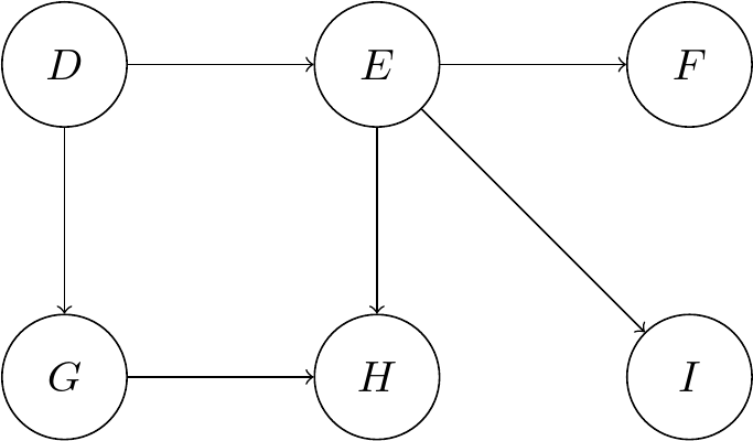
According to the earlier formula we can express the joint distribution by following the topological ordering. Simply put, we begin at a node with no parents, then continue with another one without parents if the first node was to be removed. This is repeated until we have covered all nodes.

$$p(D,E,F,G,H,I)=p(D)p(E\vert D)p(G\vert D)p(F\vert E)p(H\vert E, G)p(I\vert E)$$

We can also observe that the node $E$ d-separates the nodes $D, G, H$ from the nodes $F, I$. This means we can make the following conditional independence statements:

$$p(D,G,H \vert E, F, I) = p(D,G,H \vert E)$$

$$p(F, I \vert D, E, G, H) = p(F, I \vert E)$$

$$p(D, F, G, H, I \vert E) = p(D, G, H\vert E)p(F,I \vert E)$$

Summary

To wrap up, we looked at the basic principle of VAEs and the derivation of their loss function, including the ELBO. We also looked at directed graphical models and the concept of conditional independence. Next up, we will look at state space models and how to extend the concept of a VAEs to sequences of random variables.

References

[1] D. P. Kingma and M. Welling. Auto-Encoding Variational Bayes. arXiv preprint arXiv:1312.6114. 2013

[2] K. P. Murphy. Machine learning: a probabilistic perspective. 2012

Comments